What is Cluster analysis?
Cluster means a group, and a cluster of data means a group of data that are similar in type. This type of analysis is described more like discovery than a prediction, in which the machine searches for similarities within the data.
Cluster analysis in the data science career can be used in customer segmentation, stock market clustering, and to reduce dimensionality. It is done by grouping data with similar values. This analysis is good for business.
Supervised and Unsupervised Learning-
The simple difference between both types of learning is that the supervised method predicts the outcome, while the unsupervised method produces a new variable.
Here is an example. A dataset of the total expenditure of the customers and their age is provided. Now the company wants to send more ad emails to its customers.
library(ggplot2)
df <- data.frame(age = c(18, 21, 22, 24, 26, 26, 27, 30, 31, 35, 39, 40, 41, 42, 44, 46, 47, 48, 49, 54),
spend = c(10, 11, 22, 15, 12, 13, 14, 33, 39, 37, 44, 27, 29, 20, 28, 21, 30, 31, 23, 24)
)
ggplot(df, aes(x = age, y = spend)) +
geom_point()
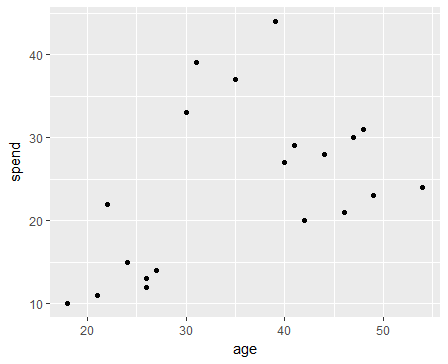
In the graph, there will be certain groups of points. In the bottom, the group of dots represents the group of young people with less money.
The topmost group represents the middle age people with higher budgets, and the rightmost group represents the old people with a lower budget.
This is one of the straightforward examples of cluster analysis.
K-means algorithm
It is a common clustering method. This algorithm reduces the distance between the observations to easily find the cluster of data. This is also known as a local optimal solutions algorithm. The distances of the observations can be measured through their coordinates.
How does the algorithm work?
- Chooses groups randomly
- The distance between the cluster center (centroid) and other observations are calculated.
- This results in a group of observations. K new clusters are formed and the observations are clustered with the closest centroid.
- The centroid is shifted to the mean coordinates of the group.
- Distances according to the new centroids are calculated. New boundaries are created, and the observations move from one group to another as they are clustered with the nearest new centroid.
- Repeat the process until no observations change their group.
The distance along x and y-axis is defined as-
D(x,y)= √ Summation of (Σ) square of (Xi-Yi). This is known as the Euclidean distance and is commonly used in the k-means algorithm. Other methods that can be used to find the distance between observations are Manhattan and Minkowski.
Select the number of clusters
The difficulty of K-means is choosing the number of clusters (k). A high k-value selected will have a large number of groups and can increase stability, but can overfit data. Overfitting is the process in which the performance of the model decreases for new data because the model has learned just the training data and this learning cannot be generalized.
The formula for choosing the number of clusters-
Cluster= √ (2/n)
Import data
K means is not suitable for factor variables. It is because the discrete values do not produce accurate predictions and it is based on the distance.
library(dplyr)
PATH <-"https://raw.githubusercontent.com/guru99-edu/R-Programming/master/computers.csv"
df <- read.csv(PATH) %>%
select(-c(X, cd, multi, premium))
glimpse(df)
Output:
Observations: 6,259
Variables: 7
$ price <int> 1499, 1795, 1595, 1849, 3295, 3695, 1720, 1995, 2225, 2575, 2195, 2605, 2045, 2295, 2699...
$ speed <int> 25, 33, 25, 25, 33, 66, 25, 50, 50, 50, 33, 66, 50, 25, 50, 50, 33, 33, 33, 66, 33, 66, ...
$ hd <int> 80, 85, 170, 170, 340, 340, 170, 85, 210, 210, 170, 210, 130, 245, 212, 130, 85, 210, 25...
$ ram <int> 4, 2, 4, 8, 16, 16, 4, 2, 8, 4, 8, 8, 4, 8, 8, 4, 2, 4, 4, 8, 4, 4, 16, 4, 8, 2, 4, 8, 1...
$ screen <int> 14, 14, 15, 14, 14, 14, 14, 14, 14, 15, 15, 14, 14, 14, 14, 14, 14, 15, 15, 14, 14, 14, ...
$ ads <int> 94, 94, 94, 94, 94, 94, 94, 94, 94, 94, 94, 94, 94, 94, 94, 94, 94, 94, 94, 94, 94, 94, ...
$ trend <int> 1, 1, 1, 1, 1, 1, 1, 1, 1, 1, 1, 1, 1, 1, 1, 1, 1, 1, 1, 1, 1, 1, 1, 1, 1, 1, 1, 1, 1, 1...
Optimal k
Elbow method is one of the methods to choose the best k value (the number of clusters). It uses in-group similarity or dissimilarity to determine the variability. Elbow graph can be constructed in the following way-
1. Create a function that computes the sum of squares of the cluster.
kmean_withinss <- function(k) {
cluster <- kmeans(rescale_df, k)
return (cluster$tot.withinss)
}
2. Run it n times
# Set maximum cluster
max_k <-20
# Run algorithm over a range of k
wss <- sapply(2:max_k, kmean_withinss)
3. Use the results to create a data frame
# Create a data frame to plot the graph
elbow <-data.frame(2:max_k, wss)
4. Plot the results
# Plot the graph with gglop
ggplot(elbow, aes(x = X2.max_k, y = wss)) +
geom_point() +
geom_line() +
scale_x_continuous(breaks = seq(1, 20, by = 1))